![]()
![]()
The goal of regport is to provides R6 classes, methods and utilities to construct, analyze, summarize, and visualize regression models (CoxPH and GLMs).
This package is been superseded by bregr.
You can install the development version of regport like so:
remotes::install_github("ShixiangWang/regport")This is a basic example which shows you how to build and visualize a Cox model.
Prepare data:
library(regport)
library(survival)

lung = survival::lung
lung$sex = factor(lung$sex)
Create a model:
model = REGModel$new(
  lung,
  recipe = list(
    x = c("age", "sex"),
    y = c("time", "status")
  )
)

model
#> <REGModel>    ==========
#>
#> Parameter | Coefficient |       SE |       95% CI |     z |     p
#> -----------------------------------------------------------------
#> age       |        1.02 | 9.38e-03 | [1.00, 1.04] |  1.85 | 0.065
#> sex [2]   |        0.60 |     0.10 | [0.43, 0.83] | -3.06 | 0.002
#>
#> Uncertainty intervals (equal-tailed) and p-values (two-tailed) computed
#>   using a Wald z-distribution approximation.
#> [coxph] model ==========
You can also create it with formula:
model = REGModel$new(
  lung,
  recipe = Surv(time, status) ~ age + sex
)

model
#> <REGModel>    ==========
#>
#> Parameter | Coefficient |       SE |       95% CI |     z |     p
#> -----------------------------------------------------------------
#> age       |        1.02 | 9.38e-03 | [1.00, 1.04] |  1.85 | 0.065
#> sex [2]   |        0.60 |     0.10 | [0.43, 0.83] | -3.06 | 0.002
#>
#> Uncertainty intervals (equal-tailed) and p-values (two-tailed) computed
#>   using a Wald z-distribution approximation.
#> [coxph] model ==========
Take a look at the model result (package see is
required):
model$plot()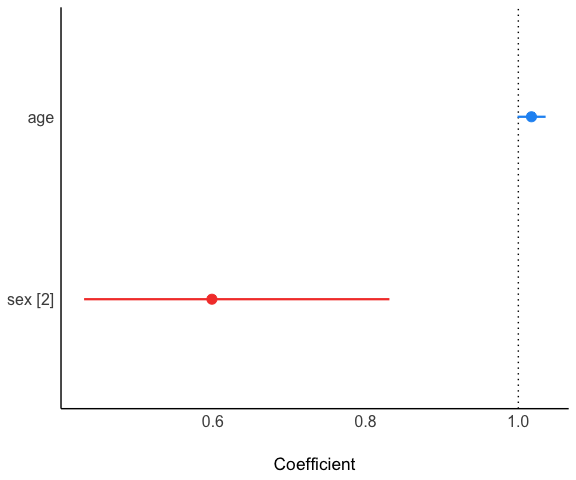
Visualize with more nice forest plot.
model$get_forest_data()
model$plot_forest()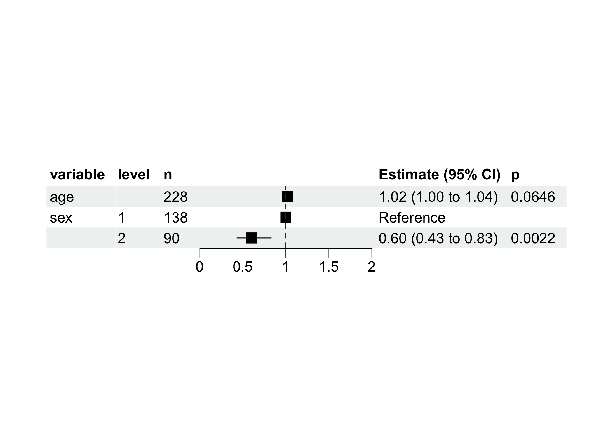
For building a list of regression model, unlike above, a lazy
building approach is used, i.e., $build() must manually
typed after creating REGModelList object. (This also means
you can check or modify the setting before building if necessary)
ml <- REGModelList$new(
  data = mtcars,
  y = "mpg",
  x = c("factor(cyl)", colnames(mtcars)[3:5]),
  covars = c(colnames(mtcars)[8:9], "factor(gear)")
)
ml
#> <REGModelList>    ==========
#>
#> X(s): factor(cyl), disp, hp, drat
#> Y(s): mpg
#> covars: vs, am, factor(gear)
#>
#> Not build yet, run $build() method
#> [] model ==========
ml$build(f = "gaussian")
str(ml$result)
#> Classes 'data.table' and 'data.frame':   25 obs. of  10 variables:
#>  $ focal_term: chr  "factor(cyl)" "factor(cyl)" "factor(cyl)" "factor(cyl)" ...
#>  $ variable  : chr  "(Intercept)" "factor(cyl)6" "factor(cyl)8" "vs" ...
#>  $ estimate  : num  23.28 -5.34 -8.5 1.68 4.31 ...
#>  $ SE        : num  3.1 1.89 3.05 2.35 2.16 ...
#>  $ CI        : num  0.95 0.95 0.95 0.95 0.95 0.95 0.95 0.95 0.95 0.95 ...
#>  $ CI_low    : num  17.203 -9.04 -14.473 -2.931 0.084 ...
#>  $ CI_high   : num  29.37 -1.64 -2.53 6.3 8.54 ...
#>  $ t         : num  7.504 -2.829 -2.791 0.715 1.999 ...
#>  $ df_error  : int  25 25 25 25 25 25 25 26 26 26 ...
#>  $ p         : num  6.18e-14 4.67e-03 5.25e-03 4.75e-01 4.56e-02 ...
#>  - attr(*, ".internal.selfref")=<externalptr>
str(ml$forest_data)
#> Classes 'data.table' and 'data.frame':   6 obs. of  17 variables:
#>  $ focal_term: chr  "factor(cyl)" "factor(cyl)" "factor(cyl)" "disp" ...
#>  $ variable  : chr  "factor(cyl)" NA NA "disp" ...
#>  $ term      : chr  "factor(cyl)4" "factor(cyl)6" "factor(cyl)8" "disp" ...
#>  $ term_label: chr  "factor(cyl)" "factor(cyl)" "factor(cyl)" "disp" ...
#>  $ class     : chr  "factor" "factor" "factor" "numeric" ...
#>  $ level     : chr  "4" "6" "8" NA ...
#>  $ level_no  : int  1 2 3 NA NA NA
#>  $ n         : int  11 7 14 32 32 32
#>  $ estimate  : num  0 -5.3404 -8.5026 -0.0282 -0.0515 ...
#>  $ SE        : num  NA 1.88767 3.04626 0.00924 0.01201 ...
#>  $ CI        : num  NA 0.95 0.95 0.95 0.95 0.95
#>  $ CI_low    : num  NA -9.0402 -14.4732 -0.0463 -0.075 ...
#>  $ CI_high   : num  NA -1.6407 -2.532 -0.0101 -0.0279 ...
#>  $ t         : num  NA -2.83 -2.79 -3.05 -4.28 ...
#>  $ df_error  : int  NA 25 25 26 26 26
#>  $ p         : num  NA 4.67e-03 5.25e-03 2.27e-03 1.84e-05 ...
#>  $ reference : logi  TRUE FALSE FALSE FALSE FALSE FALSE
#>  - attr(*, ".internal.selfref")=<externalptr>

ml$plot_forest(ref_line = 0, xlim = c(-15, 8))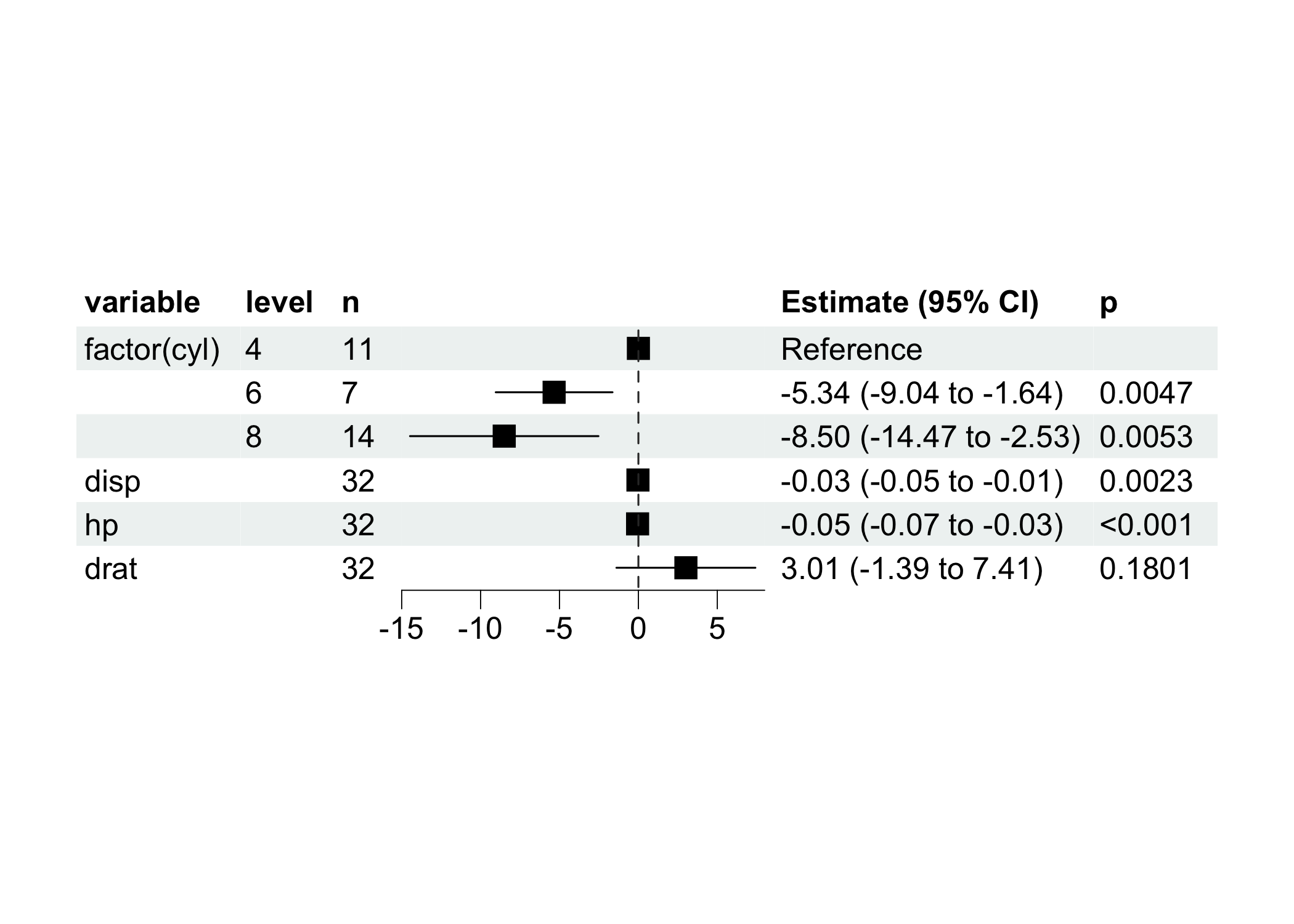
covr::package_coverage()
#> regport Coverage: 85.28%
#> R/utils.R: 75.00%
#> R/REGModelList.R: 81.91%
#> R/REGModel.R: 87.56%(MIT) Copyright (c) 2022 Shixiang Wang