The independenceWeights package constructs weights
designed to minimize the weighted statistical dependence between a
continuous exposure variable and a vector of confounder variables and
implements the methods of Huling, Greifer, and Chen (2021) for doing so.
In estimating a causal dose-response function, confounding bias is a
function of the dependence between confounders and the
exposure/treatment, so weights that minimize the dependence aim to
mitigate confounding bias directly.
Install the development version from GitHub with:
# install.packages("devtools")
devtools::install_github("jaredhuling/independenceWeights")This is a basic example which shows how to estimate and utilize the distance covariance optimal weights (DCOWs) of Huling, Greifer, and Chen (2021):
library(independenceWeights)Simulate data with a continuous treatment that has a confounded relationship with a response. Data are simulated according to the simulation setup of Vegetabile et al. (2021).
simdat <- simulate_confounded_data(seed = 999, nobs = 500)
y <- simdat$data$Y ## response
A <- simdat$data$A ## treatment
X <- as.matrix(simdat$data[c("Z1", "Z2", "Z3", "Z4", "Z5")]) ## confounders
Now estimate weights to adjust for confounders using the distance covariance optimal weights (DCOWs), which aim to mitigate the dependence between A and X:
dcows <- independence_weights(A, X)

dcows
#> Unweighted distance covariance:           0.3963
#> Optimized weighted dependence distance:   0.0246
#> Effective sample size:                  264.0099
#>
#> Weight ranges:
#>    Min. 1st Qu.  Median    Mean 3rd Qu.    Max.
#>  0.0000  0.2767  0.8215  1.0000  1.4120  5.7360
Alternatively, information about any set of weights can be printed
via weighted_energy_stats(). The unweighted distance
covariance is a measure of the unadjusted dependence between confounders
and treatment. The weighted dependence distance is a measure of this
dependence after weighting. The weighted energy distance
between A and weighted A measures how well the marginal distribution of
A is preserved after weighting. Similarly for X. The effective sample
size estimates the effective sample size after weighting.
weighted_energy_stats(A, X, dcows$weights)
#> Unweighted distance covariance:            0.3963
#> Weighted dependence distance:              0.0246
#> Weighted energy distance(A, weighted A):   0.0014
#> Weighted energy distance(X, weighted X):   0.0025
#> Effective sample size:                   264.0099
We can assess traditional measures of balance such as marginal
weighted correlations with cobalt:
library(cobalt)Even though the DCOWs aim to mitigate joint dependence between X and
A, they result in very small marginal weighted correlations between them
as well. (changing poly to 10 below would reveal that even
up to 10th degree polynomials of covariates as well-decorrelated):
bal.tab(A ~ Z1 + Z2 + Z3 + Z4 + Z5, data = data.frame(A = A, X),
        weights = list(DCOW = dcows$weights),
        un = TRUE, int = TRUE, poly = 1, stats = "cor")
#> Balance Measures
#>              Type Corr.Un Corr.Adj
#> Z1        Contin. -0.1351  -0.0021
#> Z2        Contin.  0.4445   0.0161
#> Z3        Contin. -0.0397  -0.0284
#> Z4        Contin.  0.0267  -0.0057
#> Z5         Binary  0.0691   0.0009
#> Z1 * Z2   Contin. -0.0944   0.0016
#> Z1 * Z3   Contin. -0.1539  -0.0080
#> Z1 * Z4   Contin. -0.0168  -0.0007
#> Z1 * Z5_0 Contin. -0.1445  -0.0101
#> Z1 * Z5_1 Contin.  0.0438   0.0101
#> Z2 * Z3   Contin.  0.2647  -0.0129
#> Z2 * Z4   Contin.  0.0488  -0.0027
#> Z2 * Z5_0 Contin. -0.0266  -0.0005
#> Z2 * Z5_1 Contin.  0.0884   0.0027
#> Z3 * Z4   Contin.  0.0260  -0.0077
#> Z3 * Z5_0 Contin. -0.0730  -0.0064
#> Z3 * Z5_1 Contin.  0.0669   0.0019
#> Z4 * Z5_0 Contin. -0.0016  -0.0038
#> Z4 * Z5_1 Contin.  0.0486  -0.0037
#>
#> Effective sample sizes
#>             Total
#> Unadjusted 500.
#> Adjusted   264.01
We can also minimize the weighted dependence subject to the constraint that marginal moments of X and A are decorrelated:
dcows_decor <- independence_weights(A, X,
                                    decorrelate_moments = TRUE)

dcows_decor
#> Unweighted distance covariance:           0.3963
#> Optimized weighted dependence distance:   0.0251
#> Effective sample size:                  260.8907
#>
#> Weight ranges:
#>    Min. 1st Qu.  Median    Mean 3rd Qu.    Max.
#> 0.0000 0.2491 0.8344 1.0000 1.4330 5.7290bal.tab(A ~ Z1 + Z2 + Z3 + Z4 + Z5, data = data.frame(A = A, X),
weights = list(DCOW = dcows$weights,
DCOW_decor = dcows_decor$weights),
un = TRUE, int = TRUE, stats = "cor")
#> Balance Measures
#> Type Corr.Un Corr.DCOW Corr.DCOW_decor
#> Z1 Contin. -0.1351 -0.0021 0.0000
#> Z2 Contin. 0.4445 0.0161 -0.0004
#> Z3 Contin. -0.0397 -0.0284 -0.0002
#> Z4 Contin. 0.0267 -0.0057 -0.0002
#> Z5 Binary 0.0691 0.0009 -0.0000
#> Z1 * Z2 Contin. -0.0944 0.0016 0.0023
#> Z1 * Z3 Contin. -0.1539 -0.0080 -0.0021
#> Z1 * Z4 Contin. -0.0168 -0.0007 0.0058
#> Z1 * Z5_0 Contin. -0.1445 -0.0101 -0.0087
#> Z1 * Z5_1 Contin. 0.0438 0.0101 0.0104
#> Z2 * Z3 Contin. 0.2647 -0.0129 -0.0024
#> Z2 * Z4 Contin. 0.0488 -0.0027 0.0019
#> Z2 * Z5_0 Contin. -0.0266 -0.0005 -0.0012
#> Z2 * Z5_1 Contin. 0.0884 0.0027 0.0012
#> Z3 * Z4 Contin. 0.0260 -0.0077 -0.0011
#> Z3 * Z5_0 Contin. -0.0730 -0.0064 -0.0020
#> Z3 * Z5_1 Contin. 0.0669 0.0019 0.0019
#> Z4 * Z5_0 Contin. -0.0016 -0.0038 0.0018
#> Z4 * Z5_1 Contin. 0.0486 -0.0037 -0.0032
#>
#> Effective sample sizes
#> Total
#> All 500.
#> DCOW 264.01
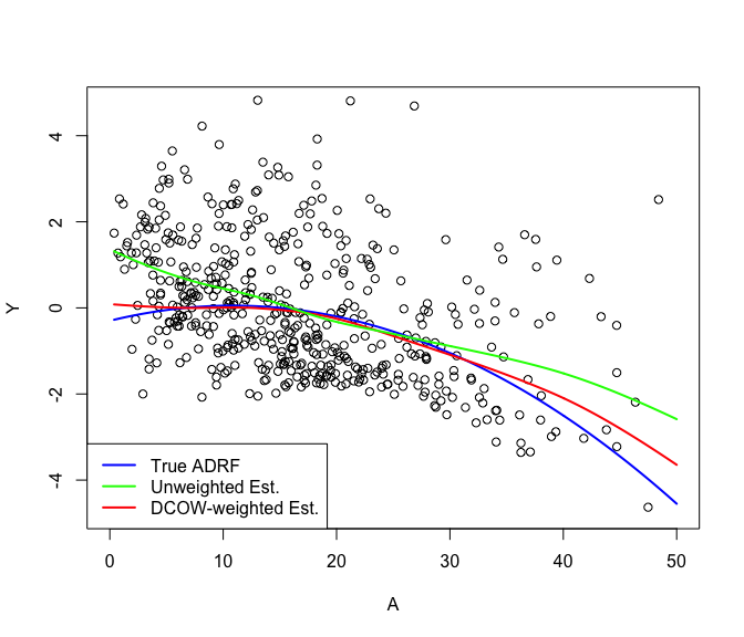
#> DCOW_decor 260.89Now use the weights to estimate the causal average dose response function (ADRF)
## create grid
trt_vec <- seq(min(simdat$data$A), 50, length.out=500)

## estimate ADRF
adrf_hat <- weighted_kernel_est(A, y, dcows$weights, trt_vec)$est

## estimate naively without weights
adrf_hat_unwtd <- weighted_kernel_est(A, y, rep(1, length(y)), trt_vec)$est

ylims <- c(-4.75, 4.75)
plot(x = simdat$data$A, y = simdat$data$Y, ylim = ylims,
     xlim = c(0,50),
     xlab = "A", ylab = "Y")
## true ADRF
lines(x = trt_vec, y = simdat$true_adrf(trt_vec), col = "blue", lwd=2)
## estimated ADRF
lines(x = trt_vec, y = adrf_hat, col = "red", lwd=2)
## naive estimate
lines(x = trt_vec, y = adrf_hat_unwtd, col = "green", lwd=2)
legend("bottomleft", c("True ADRF", "Unweighted Est.", "DCOW-weighted Est."),
       col = c("blue", "green", "red"), lty = 1, lwd = 2)