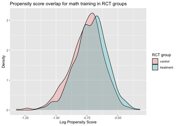
 The plot shows overlap of the density across propensity for treatment
and control group, indicating that the randomization is successful and
there is baseline balance between treatment groups.
The plot shows overlap of the density across propensity for treatment
and control group, indicating that the randomization is successful and
there is baseline balance between treatment groups.NOTE: This is a package is under construction.
The goal of WSCdata is to make a within-study comparison design data for evaluating non-experimental methods publicly available. We aim to improve access to high-quality within-study comparison data for applied methodological research.
To install the latest version of WSCdata from CRAN with:
install.packages("WSCdata")To install the development version of WSCdata from GitHub with:
# install.packages("devtools")
devtools::install_github("jzangela/WSCdata")The study aimed to examine the impact of a mathematics training
intervention and a vocabulary study session on posttest scores in
mathematics and vocabulary, respectively. The dataset
WSCdata provides baseline measures on general
self-efficacy, mathematics confidence, demographic questions, pretest
measures, selection, random assignment, and posttest measures. We
provide item-level data for the pre- and post-tests of the mathematics
and vocabulary interventions in the datasets Math_Pre_WSC,
Math_Post_WSC, Vocab_Pre_WSC, and
Vocab_Post_WSC. Additionally, item responses recorded
during mathematics training sessions are available for participants who
received the mathematics intervention in the dataset
Math_Train_WSC. Responses to non-cognitive items were also
available in their own dataset. AMAS_WSC contains item-wise
measurement data from a nine-item Abbreviated Mathematics Anxiety Scale
(Hopko et al., 2003) that assesses mathematics anxiety.
BDI_WSC includes item-wise measurement data from a
thirteen-item Beck Depression Inventory (Beck et al., 1996) that
measures symptoms of depression. Big5_WSC offers item-wise
measurement data from the Big Five Personality Inventory (John &
Srivastava, 1999) that assesses personality on five dimensions: openness
to experience, conscientiousness, extraversion, agreeableness, and
neuroticism. GSES_WSC provides item-wise measurement data
from the General Self-Efficacy Scale (Schwarzer & Jerusalem, 1995)
that measures the degree to which participants believe in their ability
to cope with unexpected or difficult situations. MSC_WSC
contains researcher-created measures on confidence in understanding of,
and ability to simplify, algebraic expressions involving exponents.
Below is an example of analysis based on WSCdata for
estimating intervention effect.
if (requireNamespace("tidyverse", quietly = TRUE)) {
  library(WSCdata)
  library(tidyverse)

  # Load WSCdata
  data("WSCdata", package = "WSCdata")
}
We first specified a list of baseline covariates in
cov_nms for future adjustments or propensity score
modeling.
# A list of covariates that will be used for further adjustment
cov_nms <- c(
  "female", "white", "black", "asian", "hisp",
  "married", "logAge", "income",
  "collegeS", "collegeM", "collegeD",
  "calc", "logBooks", "mathLike",
  "big5O", "big5C", "big5E", "big5A", "big5N",
  "AMAS", "logBDI", "MCS", "GSES",
  "vocabPre", "mathPre"
)
Here is an example of average treatment effect (ATE) estimation based on random assignment. To study the impact of a mathematics training intervention, we can use difference in mean estimation method, as shown in the following analysis
fmla_unadj_ate_math <- as.formula(paste("mathPost ~ mathGrp"))
summary(lm(fmla_unadj_ate_math, data = WSCdata))
#>
#> Call:
#> lm(formula = fmla_unadj_ate_math, data = WSCdata)
#>
#> Residuals:
#>     Min      1Q  Median      3Q     Max
#> -9.3299 -2.5695 -0.3299  2.6701  6.4305
#>
#> Coefficients:
#>             Estimate Std. Error t value Pr(>|t|)
#> (Intercept)   8.5695     0.1051   81.52  < 2e-16 ***
#> mathGrp       0.7603     0.1512    5.03  5.3e-07 ***
#> ---
#> Signif. codes:  0 '***' 0.001 '**' 0.01 '*' 0.05 '.' 0.1 ' ' 1
#>
#> Residual standard error: 3.543 on 2198 degrees of freedom
#> Multiple R-squared:  0.01138,    Adjusted R-squared:  0.01093
#> F-statistic:  25.3 on 1 and 2198 DF,  p-value: 5.302e-07
The results show that the difference-in-means estimators for the ATE estimand for the effects of mathematics intervention on its posttests is 0.76 (SE: 0.15). This indicates that the average treatment effect (ATE) of mathematics training on math test scores is 0.76.
We can further adjust for baseline covariates specified in
cov_nms in the estimation
fmla_ancova_ate_math <-
  as.formula(paste("mathPost ~ mathGrp + ", paste(cov_nms, collapse = " + ")))
summary(lm(fmla_ancova_ate_math, data = WSCdata))
#>
#> Call:
#> lm(formula = fmla_ancova_ate_math, data = WSCdata)
#>
#> Residuals:
#>     Min      1Q  Median      3Q     Max
#> -9.2772 -1.3605  0.0836  1.4372  6.9177
#>
#> Coefficients:
#>              Estimate Std. Error t value Pr(>|t|)
#> (Intercept)  4.160199   1.034178   4.023 5.95e-05 ***
#> mathGrp      0.780127   0.088821   8.783  < 2e-16 ***
#> female      -0.072388   0.097467  -0.743 0.457744
#> white        0.010217   0.196198   0.052 0.958475
#> black        0.208908   0.213851   0.977 0.328736
#> asian        0.631226   0.238121   2.651 0.008087 **
#> hisp         0.308496   0.194260   1.588 0.112419
#> married     -0.096093   0.099671  -0.964 0.335103
#> logAge      -0.955883   0.177121  -5.397 7.52e-08 ***
#> income      -0.087611   0.104823  -0.836 0.403359
#> collegeS     0.479408   0.103322   4.640 3.69e-06 ***
#> collegeM    -0.086150   0.115155  -0.748 0.454466
#> collegeD     0.147552   0.111354   1.325 0.185286
#> calc         0.330209   0.103806   3.181 0.001488 **
#> logBooks    -0.102013   0.045430  -2.245 0.024836 *
#> mathLike     0.338877   0.109882   3.084 0.002068 **
#> big5O        0.004178   0.007197   0.581 0.561597
#> big5C       -0.004523   0.008700  -0.520 0.603154
#> big5E        0.024344   0.006940   3.508 0.000461 ***
#> big5A       -0.007329   0.007966  -0.920 0.357630
#> big5N       -0.006886   0.009244  -0.745 0.456401
#> AMAS        -0.028104   0.006369  -4.413 1.07e-05 ***
#> logBDI       0.036218   0.183488   0.197 0.843543
#> MCS          0.123272   0.010466  11.778  < 2e-16 ***
#> GSES        -0.011559   0.017052  -0.678 0.497899
#> vocabPre     0.080059   0.012282   6.519 8.79e-11 ***
#> mathPre      0.653601   0.018513  35.305  < 2e-16 ***
#> ---
#> Signif. codes:  0 '***' 0.001 '**' 0.01 '*' 0.05 '.' 0.1 ' ' 1
#>
#> Residual standard error: 2.065 on 2173 degrees of freedom
#> Multiple R-squared:  0.668,  Adjusted R-squared:  0.6641
#> F-statistic: 168.2 on 26 and 2173 DF,  p-value: < 2.2e-16
Holding constant the baseline covariates via Analysis of Covariates, the ATE estimate is 0.78 (SE: 0.09).
To show the overlap of the propensity in being randomly assigned to the treatment group, we can visualize it using overlap density plot
# Define the formula for the propensity score model for math training propensity
fmla_ps_math <-
  as.formula(paste("mathGrp ~ ", paste(cov_nms, collapse = " + ")))

# Fit a logistic regression model to predict propensity scores
ps_math <- predict(glm(
  formula = fmla_ps_math,
  family = "binomial",
  data = WSCdata
), type = "response")

# Merge propensity scores to the original dataset
lps_grp_math <- data.frame(cbind(lps = log(ps_math), mathGrp = WSCdata$mathGrp))

# Create an overlap density plot based on log transformed propensity scores for treatment and control group
lps_grp_math |>
  mutate(mathGrp_fct = case_when(mathGrp == 1 ~ "treatment",
                                 mathGrp == 0 ~ "control")) |>
  ggplot(aes(x = lps, fill = mathGrp_fct)) + geom_density(alpha = 0.25) +
  xlab("Log Propensity Score") +
  ylab("Density") +
  ggtitle("Propensity score overlap for math training in RCT groups") +
  guides(fill=guide_legend(title="RCT group"))
The plot shows overlap of the density across propensity for treatment
and control group, indicating that the randomization is successful and
there is baseline balance between treatment groups.
ATE estimates for the vocabulary training can be studied in the same fashion, with changing the group indicator based on vocabulary training status, which is the opposite of math training status.
Other estimators such as ATT and ATU can be studied with group indicators generated from the combination of randomization and self-selection indicator.
For more information about the four-arm WSC design and analysis, please check out Keller et al. (2025).