twfeivdecomp is a package for decomposing the two-way
fixed effects instrumental variable (TWFEIV) estimator under staggered
instrumented difference-in-differences (DID-IV) designs.
The package decomposes the TWFEIV estimator into a weighted average of
all possible Wald-DID estimators, providing a transparent view of how
different 2x2 comparisons contribute to the overall estimate.
The decomposition can be performed both with and without time-varying controls.
You can install the development version of twfeivdecomp from GitHub:
library(devtools)
install_github("shomiyaji/twfeiv-decomp")-twfeiv_decomp(): decomposes the TWFEIV estimator into
all possible Wald-DID estimators, with or without time-varying
controls.
The package includes an example dataset simulation_data,
which is a small simulated panel dataset.
It contains 72 observations (12 units observed over 6 time periods) with
the following variables:
id: Unit identifiertime: Time period (2000–2005)instrument: Binary instrument variabletreatment: Treatment variableoutcome: Outcome variablecontrol1, control2: Additional control
variablesThis is a basic example which shows how to decompose the TWFEIV
estimator into its Wald-DID components using the
twfeivdecomp package.
library(twfeivdecomp)
decomposition_result <- twfeiv_decomp(outcome ~ treatment | instrument,
data = simulation_data,
id_var = "id",
time_var = "time",
summary_output = F)
# Decomposition result
head(decomposition_result)
#> exposed_cohort unexposed_cohort design_type Wald_DID_estimate
#> 1 2001 2002 Exposed vs Not Yet Exposed 6.666667
#> 2 2005 2002 Exposed vs Exposed Shift 10.000000
#> 3 2003 2002 Exposed vs Exposed Shift 10.000000
#> 4 2002 2001 Exposed vs Exposed Shift 10.000000
#> 5 2005 2001 Exposed vs Exposed Shift 10.000000
#> 6 2003 2001 Exposed vs Exposed Shift 10.000000
#> weight
#> 1 0.02777778
#> 2 0.02777778
#> 3 0.02777778
#> 4 0.07407407
#> 5 0.07407407
#> 6 0.11111111
# Print the summary
print_summary(data = decomposition_result, return_df = FALSE)
#> # A tibble: 3 × 3
#> design_type weight_sum Weighted_average_Wald_DID
#> <chr> <dbl> <dbl>
#> 1 Exposed vs Exposed Shift 0.333 10
#> 2 Exposed vs Not Yet Exposed 0.324 8
#> 3 Exposed vs Unexposed 0.343 8.65
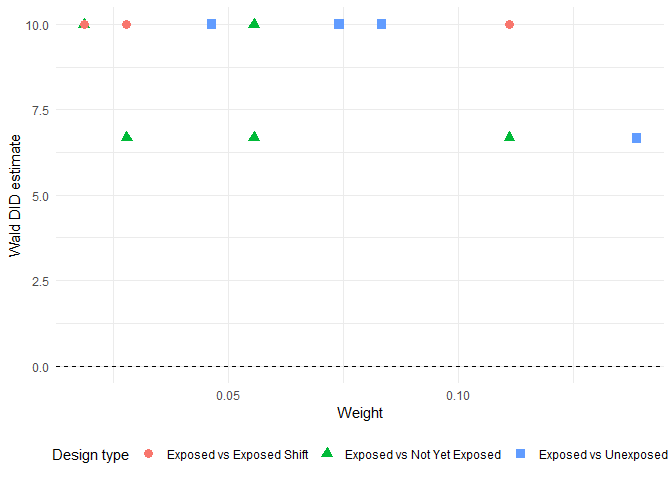
# Print the figure
library(ggplot2)
ggplot(decomposition_result) +
aes(x = weight, y = Wald_DID_estimate,
shape = factor(design_type),
color = factor(design_type)) +
geom_point(size = 3) +
geom_hline(yintercept = 0, linetype = "dashed") +
theme_minimal() +
labs(x = "Weight", y = "Wald DID estimate",
shape = "Design type", color = "Design type") +
theme(
legend.position = "bottom",
legend.box = "horizontal"
)
Miyaji, Sho. (2024). Instrumented Difference-in-Differences
with Heterogeneous Treatment Effects.
arXiv:2405.12083. Available at: https://arxiv.org/abs/2405.12083
Miyaji, Sho. (2024). Two-Way Fixed Effects Instrumental
Variable Regressions in Staggered DID-IV Designs.
arXiv:2405.16467. Available at: https://arxiv.org/abs/2405.16467