
The tidycensuskr package is designed for R users who
want to work with South Korean census and administrative boundary data.
It aims to provide an easy-to-use interface for population, housing, and
socioeconomic statistics linked with geospatial boundaries.
You can install the released version of tidycensuskr
from CRAN with:
# CRAN
install.packages("tidycensuskr")
To install the development version, you will need a GitHub account
and generate a personal access token with repo
permissions.
# Development version from GitHub
rlang::check_installed("remotes")
remotes::install_github("sigmafelix/tidycensuskr", auth_token = "__YOUR_GITHUB_TOKEN__")
After cloning the repository, you can also install the package using:
devtools::install(quick = TRUE)As of September 2025, this package contains two datasets: Census data
(censuskor) and the corresponding geospatial data.
anycensus()anycensus() allows you to query census
data for specific district or province codes and types of data
(population, tax, mortality, economy, housing) for three census years
(2010, 2015, 2020).# loading Seoul population data
tidycensuskr::anycensus(codes = "Seoul", type = "population")
#> # A tibble: 25 × 9
#> year adm1 adm1_code adm2 adm2_code type all households_total…¹
#> <int> <chr> <dbl> <chr> <dbl> <chr> <dbl>
#> 1 2020 Seoul 11 Dobong-gu 11100 populat… 312878
#> 2 2020 Seoul 11 Dongdaemun-gu 11060 populat… 332796
#> 3 2020 Seoul 11 Dongjak-gu 11200 populat… 378749
#> 4 2020 Seoul 11 Eunpyeong-gu 11120 populat… 458777
#> 5 2020 Seoul 11 Gangbuk-gu 11090 populat… 295304
#> 6 2020 Seoul 11 Gangdong-gu 11250 populat… 440022
#> 7 2020 Seoul 11 Gangnam-gu 11230 populat… 509899
#> 8 2020 Seoul 11 Gangseo-gu 11160 populat… 564114
#> 9 2020 Seoul 11 Geumcheon-gu 11180 populat… 225594
#> 10 2020 Seoul 11 Guro-gu 11170 populat… 394733
#> # ℹ 15 more rows
#> # ℹ abbreviated name: ¹`all households_total_prs`
#> # ℹ 2 more variables: `all households_male_prs` <dbl>,
#> # `all households_female_prs` <dbl>censuskordata(censuskor) loads an attached dataset
that contains the census data in long form. This dataset is
automatically loaded upon loading the package.load_district()load_district() allows you to get the
Si-Gun-Gu level sf files for the three census
years (2010, 2015, 2020).# loading boundary sf file
tidycensuskr::load_districts(year = 2020)
#> Simple feature collection with 250 features and 2 fields
#> Geometry type: GEOMETRY
#> Dimension: XY
#> Bounding box: xmin: 746111 ymin: 1463977 xmax: 1302469 ymax: 2068441
#> Projected CRS: KGD2002 / Unified CS
#> First 10 features:
#> year adm2_code geometry
#> 1 2020 21140 POLYGON ((1147104 1689056, ...
#> 2 2020 21020 POLYGON ((1137763 1683521, ...
#> 3 2020 21010 POLYGON ((1139121 1678921, ...
#> 4 2020 21040 POLYGON ((1144618 1676795, ...
#> 5 2020 21070 POLYGON ((1142639 1682655, ...
#> 6 2020 21130 POLYGON ((1147030 1688822, ...
#> 7 2020 21050 POLYGON ((1138992 1683338, ...
#> 8 2020 21030 POLYGON ((1142527 1684031, ...
#> 9 2020 21150 POLYGON ((1135430 1690583, ...
#> 10 2020 21100 MULTIPOLYGON (((1132627 167...Package vignettes are the first place to look for detailed examples. Below are some quick examples to get you started.
anycensus() will return an analysis-ready data.frame
that can be easily merged with the corresponding boundary
sf object from load_districts(). Here is a
simple example of making maps with population data.
library(tidycensuskr)
#> tidycensuskr 0.1.2 (2025-09-23)
library(ggplot2)
library(dplyr)
#>
#> Attaching package: 'dplyr'
#> The following objects are masked from 'package:stats':
#>
#>     filter, lag
#> The following objects are masked from 'package:base':
#>
#>     intersect, setdiff, setequal, union
library(tidyr)
library(sf)
#> Linking to GEOS 3.12.2, GDAL 3.11.3, PROJ 9.4.1; sf_use_s2() is TRUE
library(biscale)
library(cowplot)
sf_use_s2(FALSE)
#> Spherical geometry (s2) switched off
options(scipen = 100)

# load census data
census_pop_2020 <- anycensus(year = 2020, codes = NULL, type = "population")
#> Using character codes that are convertible to integers. Automatically converting to integers...
census_pop_2020 <- census_pop_2020 |>
  rename(population_total = `all households_total_prs`)

# load boundaries
adm2_2020 <- load_districts(year = 2020)

# merge boundaries and census data
census_2020_sf <- adm2_2020 |>
  left_join(census_pop_2020, by = c("adm2_code" = "adm2_code"))

# plot population data
census_2020_pop <-
  ggplot(census_2020_sf) +
  geom_sf(aes(fill = population_total), color = "white", size = 0.1) +
  theme_minimal() +
  labs(
    title = "Population (2020)",
    fill = "Population"
  ) +
  theme(plot.title = element_text(size = 12))

census_2020_pop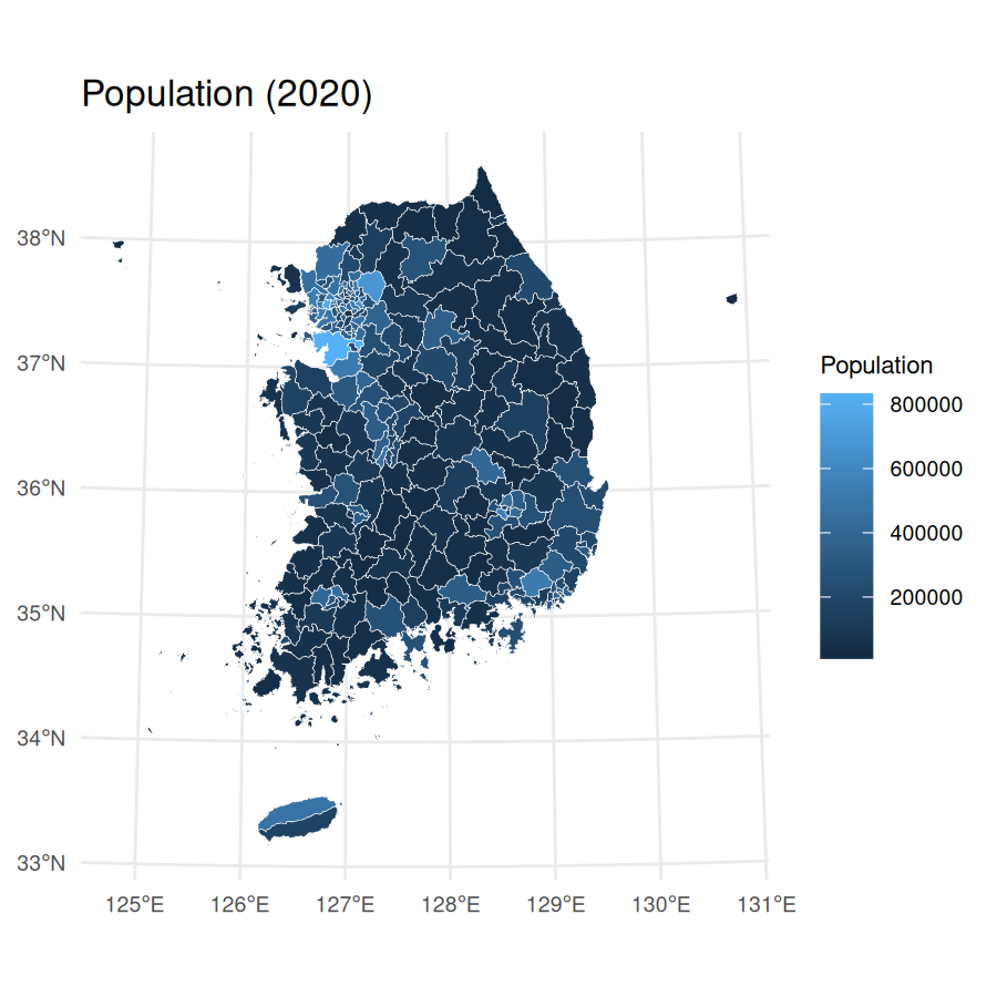
For Seoul Metropolitan Area (including Seoul, Incheon, and
Gyeonggi-do), you can use a character vector in codes
argument and merge the retrieved data.frame and
sf object with inner_join():
census_pop_2020_sma <-
  anycensus(
    year = 2020,
    codes = c("Seoul", "Incheon", "Gyeonggi"),
    type = "population"
  ) |>
  rename(population_total = `all households_total_prs`)

census_2020_sf_sma <- adm2_2020 |>
  inner_join(census_pop_2020_sma, by = c("year", "adm2_code"))


# plot population data
census_2020_pop_sma <-
  ggplot(census_2020_sf_sma) +
  geom_sf(aes(fill = population_total), color = "white", size = 0.1) +
  theme_minimal() +
  labs(
    title = "Population in Seoul Metropolitan Area (2020)",
    fill = "Population"
  ) +
  theme(plot.title = element_text(size = 12))

census_2020_pop_sma