![]()
Ridson Al Farizal P, Azka Ubaidillah
Ridson Al Farizal P ridsonap@bps.go.id
Implementation of small area estimation (Fay-Herriot model) with EBLUP (Empirical Best Linear Unbiased Prediction) Approach for non-sampled area estimation by adding cluster information and assuming that there are similarities among particular areas. See also Rao & Molina (2015, ISBN:978-1-118-73578-7) and Anisa et al. (2013) doi:10.9790/5728-10121519.
You can install the development version of saens from GitHub with:
# install.packages("devtools")
devtools::install_github("Alfrzlp/saens")
or you can install cran version
install.packages("saens")This is a basic example which shows you how to solve a common problem:
library(saens)
library(sae)
library(dplyr)
library(tidyr)
library(ggplot2)

windowsFonts(
  poppins = windowsFont('poppins')
)# Load data set from sae package
data(milk)
milk$var <- milk$SD^2
glimpse(mys)
#> Rows: 42
#> Columns: 8
#> $ area <int> 1, 2, 3, 4, 5, 6, 7, 8, 9, 10, 11, 12, 13, 14, 15, 16, 17, 18, 1…
#> $ y <dbl> 8.359527, 7.599650, 5.514137, 3.869326, 6.305063, 3.926807, 5.68…
#> $ var <dbl> 0.6618838, 0.8374691, 0.8822257, 0.6581716, 1.2788021, 0.3878004…
#> $ rse <dbl> 9.732158, 12.041783, 17.033831, 20.966899, 17.935449, 15.858590,…
#> $ x1 <dbl> 124, 89, 57, 88, 141, 96, 146, 110, 58, 63, 35, 56, 84, 240, 123…
#> $ x2 <dbl> 24, 18, 19, 35, 46, 29, 57, 41, 18, 13, 12, 14, 38, 71, 33, 53, …
#> $ x3 <dbl> 14, 9, 5, 19, 29, 10, 34, 23, 11, 5, 9, 11, 35, 48, 29, 44, 37, …
#> $ clust <dbl> 3, 3, 4, 4, 3, 4, 3, 3, 3, 3, 3, 3, 3, 4, 3, 3, 3, 3, 4, 3, 3, 3…
glimpse(milk)
#> Rows: 43
#> Columns: 7
#> $ SmallArea <int> 1, 2, 3, 4, 5, 6, 7, 8, 9, 10, 11, 12, 13, 14, 15, 16, 17, 1…
#> $ ni <int> 191, 633, 597, 221, 195, 191, 183, 188, 204, 188, 149, 290, …
#> $ yi <dbl> 1.099, 1.075, 1.105, 0.628, 0.753, 0.981, 1.257, 1.095, 1.40…
#> $ SD <dbl> 0.163, 0.080, 0.083, 0.109, 0.119, 0.141, 0.202, 0.127, 0.16…
#> $ CV <dbl> 0.148, 0.074, 0.075, 0.174, 0.158, 0.144, 0.161, 0.116, 0.12…
#> $ MajorArea <int> 1, 1, 1, 1, 1, 1, 1, 2, 2, 2, 2, 2, 2, 2, 3, 3, 3, 3, 3, 3, …
#> $ var <dbl> 0.026569, 0.006400, 0.006889, 0.011881, 0.014161, 0.019881, …model1 <- eblupfh(yi ~ as.factor(MajorArea), data = milk, vardir = "var")
#> ✔ Convergence after 4 iterations
#> → Method : REML
#>
#> ── Coefficient ─────────────────────────────────────────────────────────────────
#> beta Std.Error z-value p-value
#> (Intercept) 0.968189 0.069362 13.9585 < 2.2e-16 ***
#> as.factor(MajorArea)2 0.132780 0.103001 1.2891 0.197357
#> as.factor(MajorArea)3 0.226946 0.092330 2.4580 0.013972 *
#> as.factor(MajorArea)4 -0.241301 0.081617 -2.9565 0.003111 **
#> ---
#> Signif. codes: 0 '***' 0.001 '**' 0.01 '*' 0.05 '.' 0.1 ' ' 1AIC(model1)
#> AIC
#> -15.35496
BIC(model1)
#> BIC
#> -6.548956
logLik(model1)
#> loglike
#> 12.67748coef(model1)
#> (Intercept) as.factor(MajorArea)2 as.factor(MajorArea)3
#> 0.9681890 0.1327801 0.2269462
#> as.factor(MajorArea)4
#> -0.2413011summary(model1)
#> beta Std.Error z-value p-value
#> (Intercept) 0.968189 0.069362 13.9585 < 2.2e-16 ***
#> as.factor(MajorArea)2 0.132780 0.103001 1.2891 0.197357
#> as.factor(MajorArea)3 0.226946 0.092330 2.4580 0.013972 *
#> as.factor(MajorArea)4 -0.241301 0.081617 -2.9565 0.003111 **
#> ---
#> Signif. codes: 0 '***' 0.001 '**' 0.01 '*' 0.05 '.' 0.1 ' ' 1saens::autoplot(model1, variable = 'MSE')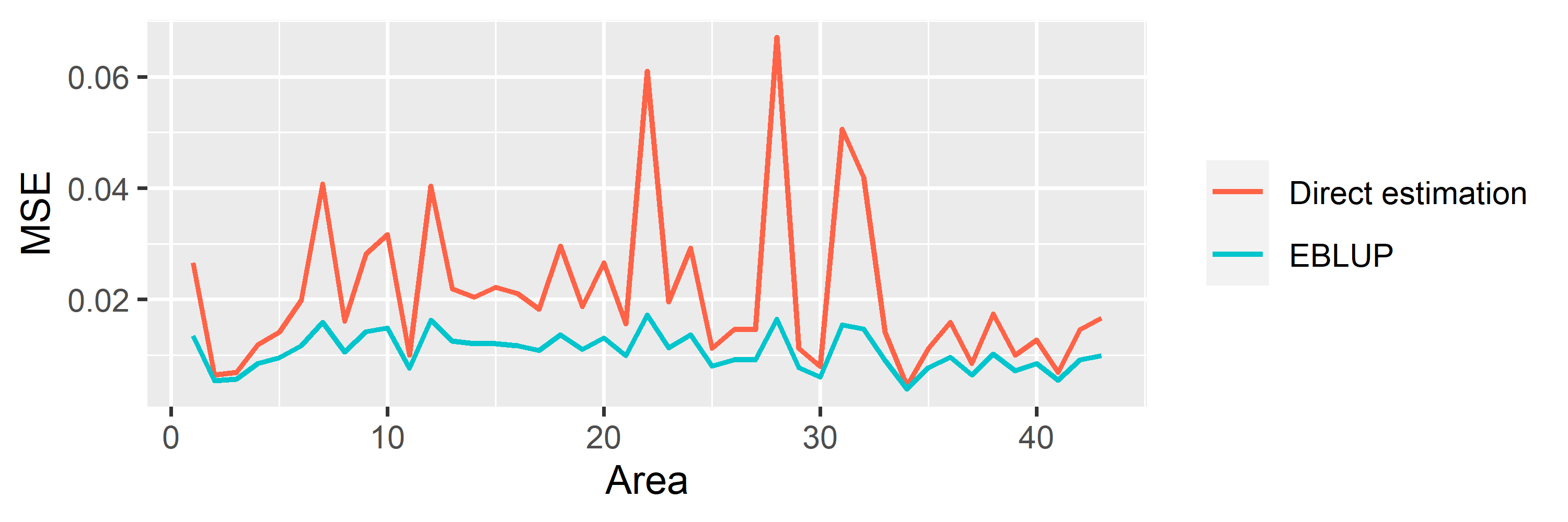
saens::autoplot(model1, variable = 'RRMSE')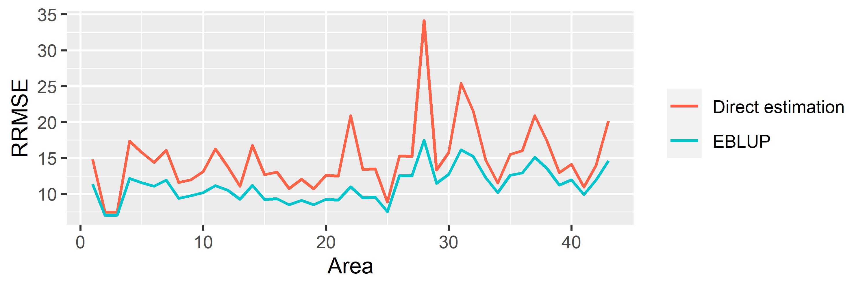
saens::autoplot(model1, variable = 'estimation')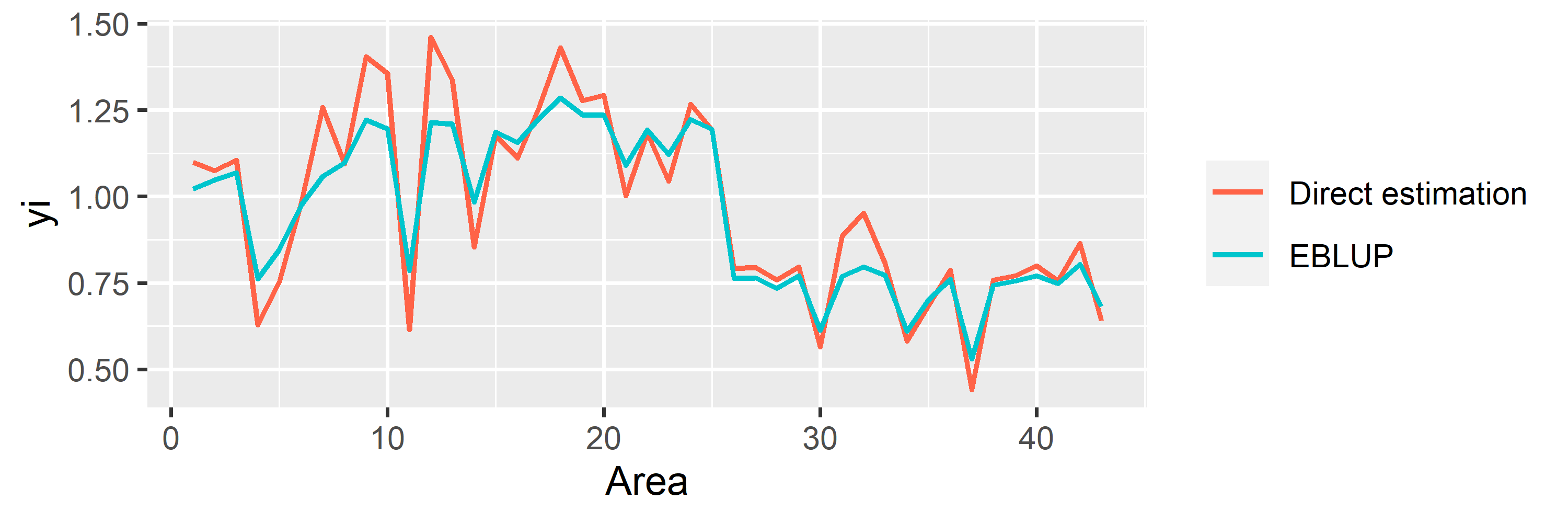
model_ns <- eblupfh_cluster(y ~ x1 + x2 + x3, data = mys, vardir = "var", cluster = "clust")
#> ✔ Convergence after 6 iterations
#> → Method : REML
#>
#> ── Coefficient ─────────────────────────────────────────────────────────────────
#>                   beta  Std.Error z-value   p-value
#> (Intercept)  3.1077510  0.7697687  4.0373 5.408e-05 ***
#> x1          -0.0019323  0.0098886 -0.1954    0.8451
#> x2           0.0555184  0.0614129  0.9040    0.3660
#> x3           0.0335344  0.0580013  0.5782    0.5632
#> ---
#> Signif. codes: 0 '***' 0.001 '**' 0.01 '*' 0.05 '.' 0.1 ' ' 1mys$eblup_est <- model_ns$df_res$eblup
mys$eblup_rse <- model_ns$df_res$rse
glimpse(mys)
#> Rows: 42
#> Columns: 10
#> $ area <int> 1, 2, 3, 4, 5, 6, 7, 8, 9, 10, 11, 12, 13, 14, 15, 16, 17, 1…
#> $ y <dbl> 8.359527, 7.599650, 5.514137, 3.869326, 6.305063, 3.926807, …
#> $ var <dbl> 0.6618838, 0.8374691, 0.8822257, 0.6581716, 1.2788021, 0.387…
#> $ rse <dbl> 9.732158, 12.041783, 17.033831, 20.966899, 17.935449, 15.858…
#> $ x1 <dbl> 124, 89, 57, 88, 141, 96, 146, 110, 58, 63, 35, 56, 84, 240,…
#> $ x2 <dbl> 24, 18, 19, 35, 46, 29, 57, 41, 18, 13, 12, 14, 38, 71, 33, …
#> $ x3 <dbl> 14, 9, 5, 19, 29, 10, 34, 23, 11, 5, 9, 11, 35, 48, 29, 44, …
#> $ clust <dbl> 3, 3, 4, 4, 3, 4, 3, 3, 3, 3, 3, 3, 3, 4, 3, 3, 3, 3, 4, 3, …
#> $ eblup_est <dbl> 7.612738, 6.782316, 5.187060, 4.201545, 6.323679, 4.048590, …
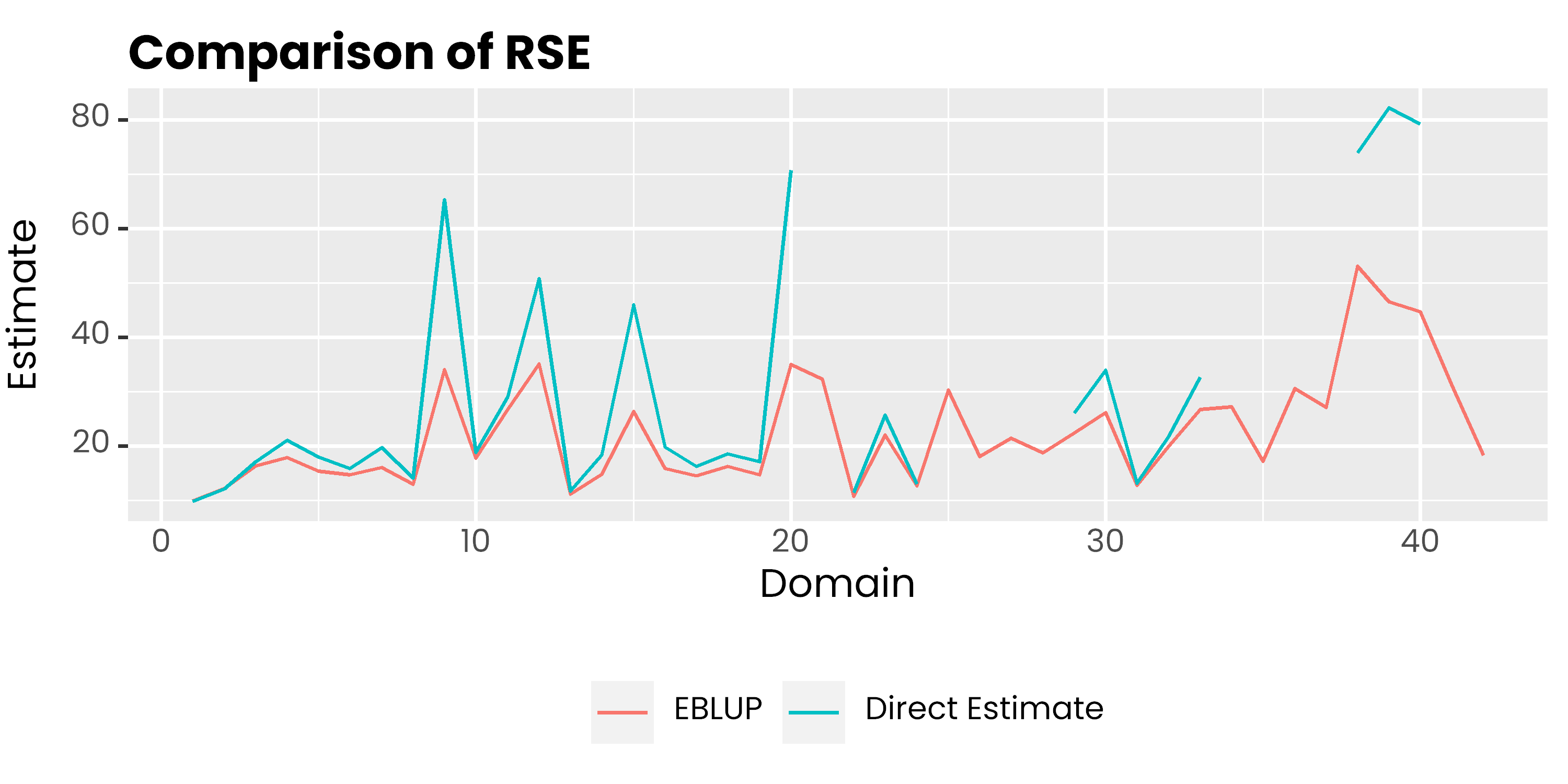
#> $ eblup_rse <dbl> 9.844182, 12.144869, 16.347620, 17.841554, 15.307573, 14.713…mys %>%
select(area, rse, eblup_rse) %>%
pivot_longer(-1, names_to = "metode", values_to = "rse") %>%
ggplot(aes(x = area, y = rse, col = metode)) +
geom_line() +
scale_color_discrete(
labels = c('EBLUP', 'Direct Estimate')
) +
labs(col = NULL, y = 'Estimate', x = 'Domain', title = 'Comparison of RSE') +
theme(
legend.position = 'bottom',
text = element_text(family = 'poppins'),
axis.ticks.x = element_blank(),
plot.title = element_text(face = 2, vjust = 0),
plot.subtitle = element_text(colour = 'gray30', vjust = 0)
)
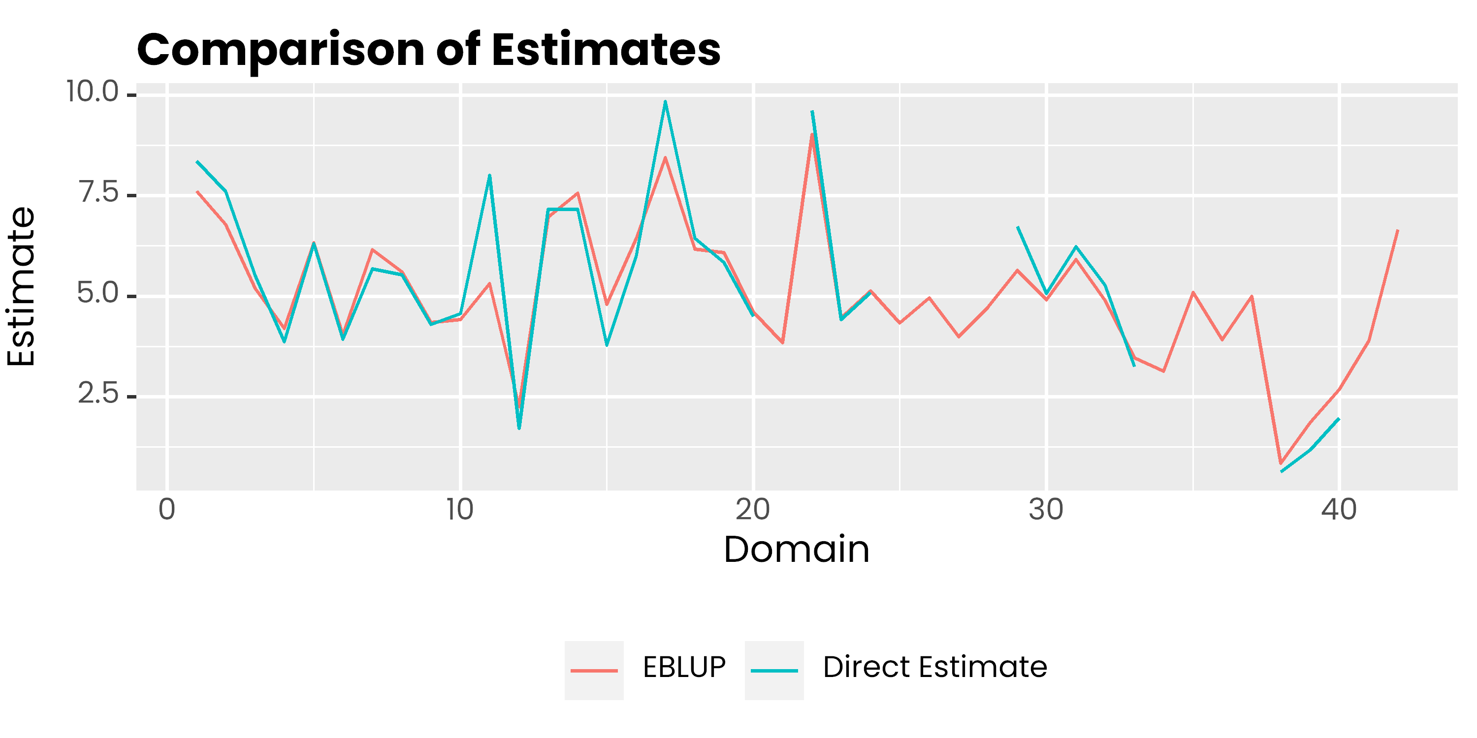
mys %>%
  select(area, y, eblup_est) %>%
  pivot_longer(-1, names_to = "metode", values_to = "rse") %>%
  ggplot(aes(x = area, y = rse, col = metode)) +
  geom_line() +
    scale_color_discrete(
    labels = c('EBLUP', 'Direct Estimate')
  ) +
  labs(col = NULL, y = 'Estimate', x = 'Domain', title = 'Comparison of Estimates') +
  theme(
    legend.position = 'bottom',
    text = element_text(family = 'poppins'),
    axis.ticks.x = element_blank(),
    plot.title = element_text(face = 2, vjust = 0),
    plot.subtitle = element_text(colour = 'gray30', vjust = 0)
  )