![]()
![]()
![]()
The goal of lotri is to easily specify block-diagonal matrices with (lo)wer (tri)angular matrices. Its as if you have won the (badly spelled) lotri (or lottery).
This was made to allow people (like me) to specify lower triangular
matrices similar to the domain specific language implemented in
nlmixr2. Originally I had it included in
RxODE, but thought it may have more general applicability,
so I separated it into a new package.
You can install the released version of lotri from CRAN with:
install.packages("lotri")And the development version from GitHub with:
# install.packages("devtools")
devtools::install_github("nlmixr2/lotri")This is a basic example for an easier way to specify matrices in R.
For instance to fully specify a simple 2x2 matrix, in R you
specify:
mat <- matrix(c(1, 0.5, 0.5, 1),nrow=2,ncol=2,dimnames=list(c("a", "b"), c("a", "b")))With lotri, you simply specify:
library(lotri)
library(microbenchmark)
library(ggplot2)


mat <- lotri(a+b ~ c(1,
                     0.5, 1))
print(mat)
#>     a   b
#> a 1.0 0.5
#> b 0.5 1.0

# You can also specify line by line:

mat <- lotri({a ~ 1
              b ~ c(0.5, 1)})
print(mat)
#>     a   b
#> a 1.0 0.5
#> b 0.5 1.0
I find it more legible and easier to specify, especially if you have a more complex matrix. For instance with the more complex matrix:
mat <- lotri({
    a+b ~ c(1,
            0.5, 1)
    c ~ 1
    d +e ~ c(1,
             0.5, 1)
})
print(mat)
#>     a   b c   d   e
#> a 1.0 0.5 0 0.0 0.0
#> b 0.5 1.0 0 0.0 0.0
#> c 0.0 0.0 1 0.0 0.0
#> d 0.0 0.0 0 1.0 0.5
#> e 0.0 0.0 0 0.5 1.0

# or
mat <- lotri({
  a ~ 1
  b ~ c(0.5, 1)
  c ~ 1
  d ~ 1
 e ~ c(0.5, 1)
})

print(mat)
#>     a   b c   d   e
#> a 1.0 0.5 0 0.0 0.0
#> b 0.5 1.0 0 0.0 0.0
#> c 0.0 0.0 1 0.0 0.0
#> d 0.0 0.0 0 1.0 0.5
#> e 0.0 0.0 0 0.5 1.0
To fully specify this in base R you would need to use:
mat <- matrix(c(1, 0.5, 0, 0, 0,
                0.5, 1, 0, 0, 0,
                0, 0, 1, 0, 0,
                0, 0, 0, 1, 0.5,
                0, 0, 0, 0.5, 1),
              nrow=5, ncol=5,
              dimnames= list(c("a", "b", "c", "d", "e"),
                             c("a", "b", "c", "d", "e")))
print(mat)
#>     a   b c   d   e
#> a 1.0 0.5 0 0.0 0.0
#> b 0.5 1.0 0 0.0 0.0
#> c 0.0 0.0 1 0.0 0.0
#> d 0.0 0.0 0 1.0 0.5
#> e 0.0 0.0 0 0.5 1.0
Of course with the excellent Matrix package this is a
bit easier:
library(Matrix)
mat <- matrix(c(1, 0.5, 0.5, 1),
              nrow=2,
              ncol=2,
              dimnames=list(c("a", "b"), c("a", "b")))

mat <- bdiag(list(mat, matrix(1), mat))

## Convert back to standard matrix
mat <- as.matrix(mat)
##
dimnames(mat) <- list(c("a", "b", "c", "d", "e"),
                      c("a", "b", "c", "d", "e"))
print(mat)
#>     a   b c   d   e
#> a 1.0 0.5 0 0.0 0.0
#> b 0.5 1.0 0 0.0 0.0
#> c 0.0 0.0 1 0.0 0.0
#> d 0.0 0.0 0 1.0 0.5
#> e 0.0 0.0 0 0.5 1.0
Regardless, I think lotri is a bit easier to use.
lotri also allows lists of matrices to be created by
conditioning on an id with the | syntax.
For example:
mat <- lotri({
    a+b ~ c(1,
            0.5, 1) | id
    c ~ 1 | occ
    d + e ~ c(1,
              0.5, 1) | id(lower=3, upper=2, omegaIsChol=FALSE)
})

print(mat)
#> $id
#>     d   e
#> d 1.0 0.5
#> e 0.5 1.0
#>
#> $occ
#>   c
#> c 1
#>
#> Properties: lower, upper, omegaIsChol

print(mat$lower)
#> $id
#> d e
#> 3 3
#>
#> $occ
#>    c
#> -Inf
print(mat$upper)
#> $id
#> d e
#> 2 2
#>
#> $occ
#>   c
#> Inf
print(mat$omegaIsChol)
#> $id
#> [1] FALSE
This gives a list of matrix(es) conditioned on the variable after the
|. It also can add properties to each list that can be
accessible after the list of matrices is returned, as shown in the above
example. To do this, you simply have to enclose the properties after the
conditional variable. That is et1 ~ id(lower=3).
Now there is even a faster way to do a similar banded matrix
concatenation with lotriMat
testList <- list(lotri({et2 + et3 + et4 ~ c(40,
                            0.1, 20,
                            0.1, 0.1, 30)}),
                     lotri(et5 ~ 6),
                     lotri(et1+et6 ~c(0.1, 0.01, 1)),
                     matrix(c(1L, 0L, 0L, 1L), 2, 2,
                            dimnames=list(c("et7", "et8"),
                                          c("et7", "et8"))))

matf <- function(.mats){
  .omega <- as.matrix(Matrix::bdiag(.mats))
  .d <- unlist(lapply(seq_along(.mats),
                      function(x) {
                        dimnames(.mats[[x]])[2]
                      }))
  dimnames(.omega) <- list(.d, .d)
  return(.omega)
}

print(matf(testList))
#>      et2  et3  et4 et5  et1  et6 et7 et8
#> et2 40.0  0.1  0.1   0 0.00 0.00   0   0
#> et3  0.1 20.0  0.1   0 0.00 0.00   0   0
#> et4  0.1  0.1 30.0   0 0.00 0.00   0   0
#> et5  0.0  0.0  0.0   6 0.00 0.00   0   0
#> et1  0.0  0.0  0.0   0 0.10 0.01   0   0
#> et6  0.0  0.0  0.0   0 0.01 1.00   0   0
#> et7  0.0  0.0  0.0   0 0.00 0.00   1   0
#> et8  0.0  0.0  0.0   0 0.00 0.00   0   1

print(lotriMat(testList))
#>      et2  et3  et4 et5  et1  et6 et7 et8
#> et2 40.0  0.1  0.1   0 0.00 0.00   0   0
#> et3  0.1 20.0  0.1   0 0.00 0.00   0   0
#> et4  0.1  0.1 30.0   0 0.00 0.00   0   0
#> et5  0.0  0.0  0.0   6 0.00 0.00   0   0
#> et1  0.0  0.0  0.0   0 0.10 0.01   0   0
#> et6  0.0  0.0  0.0   0 0.01 1.00   0   0
#> et7  0.0  0.0  0.0   0 0.00 0.00   1   0
#> et8  0.0  0.0  0.0   0 0.00 0.00   0   1

mb <- microbenchmark(matf(testList),lotriMat(testList))

print(mb)
#> Unit: microseconds
#>                expr     min      lq       mean   median        uq      max neval
#>      matf(testList) 974.141 995.431 1095.86074 1010.043 1029.2245 5398.306   100
#>  lotriMat(testList)   2.525   3.126    4.93906    5.015    5.5655   26.170   100

autoplot(mb)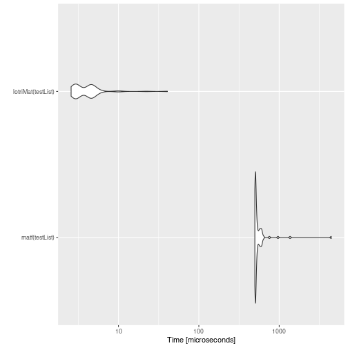
You may also combine named and unnamed matrices, but the resulting
matrix will be unnamed, and still be faster than
Matrix:
testList <- list(lotri({et2 + et3 + et4 ~ c(40,
                            0.1, 20,
                            0.1, 0.1, 30)}),
                     lotri(et5 ~ 6),
                     lotri(et1+et6 ~c(0.1, 0.01, 1)),
                     matrix(c(1L, 0L, 0L, 1L), 2, 2))

matf <- function(.mats){
  .omega <- as.matrix(Matrix::bdiag(.mats))
  return(.omega)
}

print(matf(testList))
#>      [,1] [,2] [,3] [,4] [,5] [,6] [,7] [,8]
#> [1,] 40.0  0.1  0.1    0 0.00 0.00    0    0
#> [2,]  0.1 20.0  0.1    0 0.00 0.00    0    0
#> [3,]  0.1  0.1 30.0    0 0.00 0.00    0    0
#> [4,]  0.0  0.0  0.0    6 0.00 0.00    0    0
#> [5,]  0.0  0.0  0.0    0 0.10 0.01    0    0
#> [6,]  0.0  0.0  0.0    0 0.01 1.00    0    0
#> [7,]  0.0  0.0  0.0    0 0.00 0.00    1    0
#> [8,]  0.0  0.0  0.0    0 0.00 0.00    0    1

print(lotriMat(testList))
#>      [,1] [,2] [,3] [,4] [,5] [,6] [,7] [,8]
#> [1,] 40.0  0.1  0.1    0 0.00 0.00    0    0
#> [2,]  0.1 20.0  0.1    0 0.00 0.00    0    0
#> [3,]  0.1  0.1 30.0    0 0.00 0.00    0    0
#> [4,]  0.0  0.0  0.0    6 0.00 0.00    0    0
#> [5,]  0.0  0.0  0.0    0 0.10 0.01    0    0
#> [6,]  0.0  0.0  0.0    0 0.01 1.00    0    0
#> [7,]  0.0  0.0  0.0    0 0.00 0.00    1    0
#> [8,]  0.0  0.0  0.0    0 0.00 0.00    0    1

mb <- microbenchmark(matf(testList),lotriMat(testList))

print(mb)
#> Unit: microseconds
#>                expr     min       lq       mean   median      uq      max neval
#>      matf(testList) 930.859 946.7345 1030.87673 959.0675 990.947 4007.812   100
#>  lotriMat(testList)   2.174   2.9610    4.61355   4.7390   5.526   13.916   100

autoplot(mb)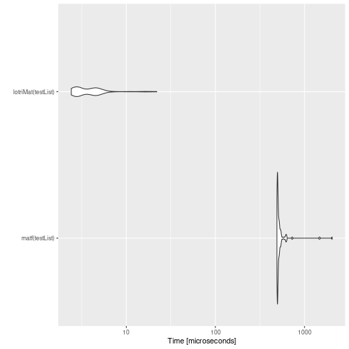
A new feature is the ability to condition on variables by
|. This will be useful when simulating nested random
effects using the upcoming RxODE2