bulkreadr

The Ultimate Tool for Reading Data in Bulk

R-CMD-check CRAN_Status_Badge metacran downloads Codecov test coverage

About the package

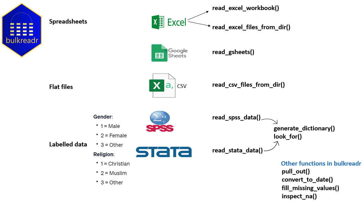
bulkreadr is an R package designed to simplify and streamline the process of reading and processing large volumes of data. With a collection of functions tailored for bulk data operations, the package allows users to efficiently read multiple sheets from Microsoft Excel/Google Sheets workbooks and multiple CSV files from a directory. It returns the data as organized data frames, making it convenient for further analysis and manipulation. Whether dealing with extensive data sets or batch processing tasks, “bulkreadr” empowers users to effortlessly handle data in bulk, saving time and effort in data preparation workflows.

Installation

You can install bulkreadr package from CRAN with:

install.packages("bulkreadr")

or the development version from GitHub with

if(!require("devtools")){
 install.packages("devtools")
}

devtools::install_github("gbganalyst/bulkreadr")

How to load the package

Now that you have installed bulkreadr package, you can simply load it by using:

library(bulkreadr)
library(dplyr)

Functions in bulkreadr package

This section provides a concise overview of the different functions available in the bulkreadr package. These functions serve various purposes and are designed to handle importing of data in bulk.

Other functions in bulkreadr package:

Note:

For the majority of functions within this package, we will utilize data stored in the system file by the bulkreadr, which can be accessed using the system.file() function. If you wish to utilize your own data stored in your local directory, please ensure that you have set the appropriate file path prior to using any functions provided by the bulkreadr package.

read_excel_workbook()

read_excel_workbook() reads all the data from the sheets of an Excel workbook and return an appended dataframe.


# path to the xls/xlsx file.

path <- system.file("extdata", "Diamonds.xlsx", package = "bulkreadr", mustWork = TRUE)

# read the sheets

read_excel_workbook(path = path)
#> # A tibble: 260 × 9
#>   carat color clarity depth table price     x     y     z
#>   <dbl> <chr> <chr>   <dbl> <dbl> <dbl> <dbl> <dbl> <dbl>
#> 1  2    I     SI1      65.9    60 13764  7.8   7.73  5.12
#> 2  0.7  H     SI1      65.2    58  2048  5.49  5.55  3.6 
#> 3  1.51 E     SI1      58.4    70 11102  7.55  7.39  4.36
#> 4  0.7  D     SI2      65.5    57  1806  5.56  5.43  3.6 
#> 5  0.35 F     VVS1     54.6    59  1011  4.85  4.79  2.63
#> # ℹ 255 more rows

read_excel_files_from_dir()

read_excel_files_from_dir() reads all Excel workbooks in the "~/data" directory and returns an appended dataframe.


# path to the directory containing the xls/xlsx files.

directory <- system.file("xlsxfolder",  package = "bulkreadr")

# import the workbooks

read_excel_files_from_dir(dir_path = directory)
#> # A tibble: 260 × 10
#>   cut   carat color clarity depth table price     x     y     z
#>   <chr> <dbl> <chr> <chr>   <dbl> <dbl> <dbl> <dbl> <dbl> <dbl>
#> 1 Fair   2    I     SI1      65.9    60 13764  7.8   7.73  5.12
#> 2 Fair   0.7  H     SI1      65.2    58  2048  5.49  5.55  3.6 
#> 3 Fair   1.51 E     SI1      58.4    70 11102  7.55  7.39  4.36
#> 4 Fair   0.7  D     SI2      65.5    57  1806  5.56  5.43  3.6 
#> 5 Fair   0.35 F     VVS1     54.6    59  1011  4.85  4.79  2.63
#> # ℹ 255 more rows

read_csv_files_from_dir()

read_csv_files_from_dir() reads all csv files from the "~/data" directory and returns an appended dataframe. The resulting dataframe will be in the same order as the CSV files in the directory.

# path to the directory containing the CSV files.

directory <- system.file("csvfolder",  package = "bulkreadr")

# import the csv files

read_csv_files_from_dir(dir_path = directory)
#> # A tibble: 260 × 10
#>   cut   carat color clarity depth table price     x     y     z
#>   <chr> <dbl> <chr> <chr>   <dbl> <dbl> <dbl> <dbl> <dbl> <dbl>
#> 1 Fair   2    I     SI1      65.9    60 13764  7.8   7.73  5.12
#> 2 Fair   0.7  H     SI1      65.2    58  2048  5.49  5.55  3.6 
#> 3 Fair   1.51 E     SI1      58.4    70 11102  7.55  7.39  4.36
#> 4 Fair   0.7  D     SI2      65.5    57  1806  5.56  5.43  3.6 
#> 5 Fair   0.35 F     VVS1     54.6    59  1011  4.85  4.79  2.63
#> # ℹ 255 more rows

read_gsheets()

The read_gsheets() function imports data from multiple sheets in a Google Sheets spreadsheet and appends the resulting dataframes from each sheet together to create a single dataframe. This function is a powerful tool for data analysis, as it allows you to easily combine data from multiple sheets into a single dataset.


# Google Sheet ID or the link to the sheet

sheet_id <- "1izO0mHu3L9AMySQUXGDn9GPs1n-VwGFSEoAKGhqVQh0"

# read all the sheets

read_gsheets(ss = sheet_id)
#> # A tibble: 260 × 9
#>   carat color clarity depth table price     x     y     z
#>   <dbl> <chr> <chr>   <dbl> <dbl> <dbl> <dbl> <dbl> <dbl>
#> 1  2    I     SI1      65.9    60 13764  7.8   7.73  5.12
#> 2  0.7  H     SI1      65.2    58  2048  5.49  5.55  3.6 
#> 3  1.51 E     SI1      58.4    70 11102  7.55  7.39  4.36
#> 4  0.7  D     SI2      65.5    57  1806  5.56  5.43  3.6 
#> 5  0.35 F     VVS1     54.6    59  1011  4.85  4.79  2.63
#> # ℹ 255 more rows

read_spss_data()

read_spss_data() is designed to seamlessly import data from an SPSS data (.sav or .zsav) files. It converts labelled variables into factors, a crucial step that enhances the ease of data manipulation and analysis within the R programming environment.


# Read an SPSS data file without converting variable labels as column names

file_path <- system.file("extdata", "Wages.sav", package = "bulkreadr")

data <- read_spss_data(file = file_path)

data
#> # A tibble: 400 × 9
#>      id  educ south                  sex   exper  wage occup marr        ed     
#>   <dbl> <dbl> <fct>                  <fct> <dbl> <dbl> <fct> <fct>       <fct>  
#> 1     3    12 does not live in South Male     17  7.5  Other Married     High s…
#> 2     4    13 does not live in South Male      9 13.1  Other Not married Some c…
#> 3     5    10 lives in South         Male     27  4.45 Other Not married Less t…
#> 4    12     9 lives in South         Male     30  6.25 Other Not married Less t…
#> 5    13     9 lives in South         Male     29 20.0  Other Married     Less t…
#> # ℹ 395 more rows

# Read an SPSS data file and convert variable labels as column names

data <- read_spss_data(file = file_path, label = TRUE)

data
#> # A tibble: 400 × 9
#>   `Worker ID` `Number of years of education` `Live in south`        Gender
#>         <dbl>                          <dbl> <fct>                  <fct> 
#> 1           3                             12 does not live in South Male  
#> 2           4                             13 does not live in South Male  
#> 3           5                             10 lives in South         Male  
#> 4          12                              9 lives in South         Male  
#> 5          13                              9 lives in South         Male  
#> # ℹ 395 more rows
#> # ℹ 5 more variables: `Number of years of work experience` <dbl>,
#> #   `Wage (dollars per hour)` <dbl>, Occupation <fct>, `Marital status` <fct>,
#> #   `Highest education level` <fct>

read_stata_data()

read_stata_data() reads Stata data file (.dta) into an R data frame, converting labeled variables into factors.

Read the Stata data file without converting variable labels as column names


file_path <- system.file("extdata", "Wages.dta", package = "bulkreadr")

data <- read_stata_data(file = file_path)

data
#> # A tibble: 400 × 9
#>      id  educ south                  sex   exper  wage occup marr        ed     
#>   <dbl> <dbl> <fct>                  <fct> <dbl> <dbl> <fct> <fct>       <fct>  
#> 1     3    12 does not live in South Male     17  7.5  Other Married     High s…
#> 2     4    13 does not live in South Male      9 13.1  Other Not married Some c…
#> 3     5    10 lives in South         Male     27  4.45 Other Not married Less t…
#> 4    12     9 lives in South         Male     30  6.25 Other Not married Less t…
#> 5    13     9 lives in South         Male     29 20.0  Other Married     Less t…
#> # ℹ 395 more rows

Read the Stata data file and convert variable labels as column names


data <- read_stata_data(file = file_path, label = TRUE)

data
#> # A tibble: 400 × 9
#>   `Worker ID` `Number of years of education` `Live in south`        Gender
#>         <dbl>                          <dbl> <fct>                  <fct> 
#> 1           3                             12 does not live in South Male  
#> 2           4                             13 does not live in South Male  
#> 3           5                             10 lives in South         Male  
#> 4          12                              9 lives in South         Male  
#> 5          13                              9 lives in South         Male  
#> # ℹ 395 more rows
#> # ℹ 5 more variables: `Number of years of work experience` <dbl>,
#> #   `Wage (dollars per hour)` <dbl>, Occupation <fct>, `Marital status` <fct>,
#> #   `Highest education level` <fct>

generate_dictionary()

generate_dictionary() creates a data dictionary from a specified data frame. This function is particularly useful for understanding and documenting the structure of your dataset, similar to data dictionaries in Stata or SPSS.


# Creating a data dictionary from an SPSS file

file_path <- system.file("extdata", "Wages.sav", package = "bulkreadr")

wage_data <- read_spss_data(file = file_path)

generate_dictionary(wage_data)
#> # A tibble: 9 × 6
#>   position variable description                     `column type` missing levels
#>      <int> <chr>    <chr>                           <chr>           <int> <name>
#> 1        1 id       Worker ID                       dbl                 0 <NULL>
#> 2        2 educ     Number of years of education    dbl                 0 <NULL>
#> 3        3 south    Live in south                   fct                 0 <chr> 
#> 4        4 sex      Gender                          fct                 0 <chr> 
#> 5        5 exper    Number of years of work experi… dbl                 0 <NULL>
#> # ℹ 4 more rows

look_for()

The look_for() function is designed to emulate the functionality of the Stata lookfor command in R. It provides a powerful tool for searching through large datasets, specifically targeting variable names, variable label descriptions, factor levels, and value labels. This function is handy for users working with extensive and complex datasets, enabling them to quickly and efficiently locate the variables of interest.


# Look for a single keyword.

look_for(wage_data, "south")
#>  pos variable label         col_type missing values                
#>  3   south    Live in south fct      0       does not live in South
#>                                              lives in South

look_for(wage_data, "e")
#>  pos variable label                              col_type missing
#>  1   id       Worker ID                          dbl      0      
#>  2   educ     Number of years of education       dbl      0      
#>  3   south    Live in south                      fct      0      
#>                                                                  
#>  4   sex      Gender                             fct      0      
#>                                                                  
#>  5   exper    Number of years of work experience dbl      0      
#>  6   wage     Wage (dollars per hour)            dbl      0      
#>  7   occup    Occupation                         fct      0      
#>                                                                  
#>                                                                  
#>                                                                  
#>                                                                  
#>                                                                  
#>  8   marr     Marital status                     fct      0      
#>                                                                  
#>  9   ed       Highest education level            fct      0      
#>                                                                  
#>                                                                  
#>                                                                  
#>                                                                  
#>  values                
#>                        
#>                        
#>  does not live in South
#>  lives in South        
#>  Male                  
#>  Female                
#>                        
#>                        
#>  Management            
#>  Sales                 
#>  Clerical              
#>  Service               
#>  Professional          
#>  Other                 
#>  Not married           
#>  Married               
#>  Less than h.s. degree 
#>  High school degree    
#>  Some college          
#>  College degree        
#>  Graduate school

pull_out()

pull_out() is similar to [. It acts on vectors, matrices, arrays and lists to extract or replace parts. It is pleasant to use with the magrittr (⁠%>%⁠) and base(|>) operators.


top_10_richest_nig <- c("Aliko Dangote", "Mike Adenuga", "Femi Otedola", "Arthur Eze", "Abdulsamad Rabiu", "Cletus Ibeto", "Orji Uzor Kalu", "ABC Orjiakor", "Jimoh Ibrahim", "Tony Elumelu")

top_10_richest_nig %>% 
  pull_out(c(1, 5, 2))
#> [1] "Aliko Dangote"    "Abdulsamad Rabiu" "Mike Adenuga"
top_10_richest_nig %>% 
  pull_out(-c(1, 5, 2))
#> [1] "Femi Otedola"   "Arthur Eze"     "Cletus Ibeto"   "Orji Uzor Kalu"
#> [5] "ABC Orjiakor"   "Jimoh Ibrahim"  "Tony Elumelu"

convert_to_date()

convert_to_date() parses an input vector into POSIXct date-time object. It is also powerful to convert from excel date number like 42370 into date value like 2016-01-01.


## ** heterogeneous dates **

dates <- c(
  44869, "22.09.2022", NA, "02/27/92", "01-19-2022",
  "13-01-  2022", "2023", "2023-2", 41750.2, 41751.99,
  "11 07 2023", "2023-4"
  )

# Convert to POSIXct or Date object

convert_to_date(dates)
#>  [1] "2022-11-04" "2022-09-22" NA           "1992-02-27" "2022-01-19"
#>  [6] "2022-01-13" "2023-01-01" "2023-02-01" "2014-04-21" "2014-04-22"
#> [11] "2023-07-11" "2023-04-01"

# It can also convert date time object to date object 

convert_to_date(lubridate::now())
#> [1] "2023-11-16"

inspect_na()

inspect_na() summarizes the rate of missingness in each column of a data frame. For a grouped data frame, the rate of missingness is summarized separately for each group.


# dataframe summary

inspect_na(airquality)
#> # A tibble: 6 × 3
#>   col_name   cnt  pcnt
#>   <chr>    <int> <dbl>
#> 1 Ozone       37 24.2 
#> 2 Solar.R      7  4.58
#> 3 Wind         0  0   
#> 4 Temp         0  0   
#> 5 Month        0  0   
#> # ℹ 1 more row

# grouped dataframe summary

airquality %>% 
  group_by(Month) %>% 
  inspect_na()
#> # A tibble: 25 × 4
#> # Groups:   Month [5]
#>   Month col_name   cnt  pcnt
#>   <int> <chr>    <int> <dbl>
#> 1     5 Ozone        5  16.1
#> 2     5 Solar.R      4  12.9
#> 3     5 Wind         0   0  
#> 4     5 Temp         0   0  
#> 5     5 Day          0   0  
#> # ℹ 20 more rows

fill_missing_values()

fill_missing_values() in an efficient function that addresses missing values in a dataframe. It uses imputation by function, meaning it replaces missing data in numeric variables with either the mean or the median, and in non-numeric variables with the mode. The function takes a column-based imputation approach, ensuring that replacement values are derived from the respective columns, resulting in accurate and consistent data. This method enhances the integrity of the dataset and promotes sound decision-making and analysis in data processing workflows.


df <- tibble::tibble(
  Sepal_Length = c(5.2, 5, 5.7, NA, 6.2, 6.7, 5.5),
  Sepal.Width = c(4.1, 3.6, 3, 3, 2.9, 2.5, 2.4),
  Petal_Length = c(1.5, 1.4, 4.2, 1.4, NA, 5.8, 3.7),
  Petal_Width = c(NA, 0.2, 1.2, 0.2, 1.3, 1.8, NA),
  Species = c("setosa", NA, "versicolor", "setosa",
    NA, "virginica", "setosa"
  )
)

df
#> # A tibble: 7 × 5
#>   Sepal_Length Sepal.Width Petal_Length Petal_Width Species   
#>          <dbl>       <dbl>        <dbl>       <dbl> <chr>     
#> 1          5.2         4.1          1.5        NA   setosa    
#> 2          5           3.6          1.4         0.2 <NA>      
#> 3          5.7         3            4.2         1.2 versicolor
#> 4         NA           3            1.4         0.2 setosa    
#> 5          6.2         2.9         NA           1.3 <NA>      
#> # ℹ 2 more rows

# Using mean to fill missing values for numeric variables

result_df_mean <- fill_missing_values(df, use_mean = TRUE)

result_df_mean
#> # A tibble: 7 × 5
#>   Sepal_Length Sepal.Width Petal_Length Petal_Width Species   
#>          <dbl>       <dbl>        <dbl>       <dbl> <chr>     
#> 1         5.2          4.1          1.5        0.94 setosa    
#> 2         5            3.6          1.4        0.2  setosa    
#> 3         5.7          3            4.2        1.2  versicolor
#> 4         5.72         3            1.4        0.2  setosa    
#> 5         6.2          2.9          3          1.3  setosa    
#> # ℹ 2 more rows

# Using median to fill missing values for numeric variables

result_df_median <- fill_missing_values(df, use_mean = FALSE)

result_df_median
#> # A tibble: 7 × 5
#>   Sepal_Length Sepal.Width Petal_Length Petal_Width Species   
#>          <dbl>       <dbl>        <dbl>       <dbl> <chr>     
#> 1          5.2         4.1          1.5         1.2 setosa    
#> 2          5           3.6          1.4         0.2 setosa    
#> 3          5.7         3            4.2         1.2 versicolor
#> 4          5.6         3            1.4         0.2 setosa    
#> 5          6.2         2.9          2.6         1.3 setosa    
#> # ℹ 2 more rows

Impute missing values (NAs) in a grouped data frame

You can use the fill_missing_values() in a grouped data frame by using other grouping and map functions. Here is an example of how to do this:

sample_iris <- tibble::tibble(
Sepal_Length = c(5.2, 5, 5.7, NA, 6.2, 6.7, 5.5),
Petal_Length = c(1.5, 1.4, 4.2, 1.4, NA, 5.8, 3.7),
Petal_Width = c(0.3, 0.2, 1.2, 0.2, 1.3, 1.8, NA),
Species = c("setosa", "setosa", "versicolor", "setosa",
          "virginica", "virginica", "setosa")
)

sample_iris
#> # A tibble: 7 × 4
#>   Sepal_Length Petal_Length Petal_Width Species   
#>          <dbl>        <dbl>       <dbl> <chr>     
#> 1          5.2          1.5         0.3 setosa    
#> 2          5            1.4         0.2 setosa    
#> 3          5.7          4.2         1.2 versicolor
#> 4         NA            1.4         0.2 setosa    
#> 5          6.2         NA           1.3 virginica 
#> # ℹ 2 more rows

sample_iris %>%
  group_by(Species) %>%
  group_split() %>%
  map_df(fill_missing_values)
#> # A tibble: 7 × 4
#>   Sepal_Length Petal_Length Petal_Width Species   
#>          <dbl>        <dbl>       <dbl> <chr>     
#> 1         5.2           1.5       0.3   setosa    
#> 2         5             1.4       0.2   setosa    
#> 3         5.23          1.4       0.2   setosa    
#> 4         5.5           3.7       0.233 setosa    
#> 5         5.7           4.2       1.2   versicolor
#> # ℹ 2 more rows

Context

bulkreadr draws on and complements / emulates other packages such as readxl, readr, and googlesheets4 to read bulk data in R.